Modeling Introduction
What are models?
When asked this same question, a group of GLOBE Carbon Cycle teachers defined models in their own words:
“A model is a tool used to refine our understanding of the world, ask new questions, and make informed predictions.”
“A model is a small or large-scale representation of a process that occurs on earth that might be hard for us to study on its natural smaller or larger scale.”
“A model is a replica of an object or concept that helps increase our understanding.”
“A model is a representation of reality that can take many forms, physical, conceptual and/or mathematical. It has some characteristics of reality, but has other characteristics that won’t match reality. Models are often used for testing purposes to evaluate different scenarios.”
These are all helpful definitions. For the GLOBE Carbon Cycle Program we define models as tools that help us understand, explain, and predict systems that are too complex or difficult to observe or comprehend on our own.
We often think that models must include complicated mathematical functions, but we can learn a great deal about systems, especially environmental systems, using simple models that require only the basic math functions such as addition, subtraction, multiplication and division.
Why use models?
Models are particularly useful in the study of environmental systems. Scientists use models to examine the fundamental behavior of a system, such as carbon storage in a forest. By knowing more about the system and understanding where knowledge is incomplete, scientists can generate hypotheses to guide future research. For example, the carbon storage in aboveground tree parts (leaves, branches, stems) has been successfully modeled based on millions of measurements. On the other hand, forest models have shown that there isn’t enough detailed information available about the belowground parts (coarse and fine roots) for scientists to fully understand how carbon storage below the ground changes over time.
Models are also useful to predict future conditions. Although such predictions are not necessarily what will happen, they can provide a range of possibilities that help scientists refine their research and help policy makers create action plans to prevent any undesirable outcomes. Building on the previous examples, how might carbon uptake and storage in forest ecosystems change if there is an increase in temperature over the next twenty years?
The Basics
Before we begin it is important to understand some basic modeling concepts and terms …
- Pool (also known as stock or reservoir): A pool is the storehouse or accumulation of material, such as carbon.
- Flux (also known as flow): The movement of material from one pool to another, per unit time. (Fluxes are often some kind of process, such as photosynthesis or evaporation.)
- Input: The flow of material entering a pool
- Output: The flow of material leaving a pool
- Turnover rate: The fraction of material in a pool that enters or leaves in a specified time interval. Turnover rate is the mathematical inverse of residence time.
- Residence time: The average length of time material spends in a given pool. Residence time depends on the rates of inflow and outflow and on the size of the pool. Residence time is the mathematical inverse of turnover rate.
- Steady state (also know as equilibrium): A condition in which the amount of material within the pool at any time remains the same. In other words, the rate of input equals the rate of output, causing the total pool size to remain unchanging in time.
More on the Basics
Let’s put the basics into practice. Consider a very small lake.
The lake is the pool. The pool contains 1000 liters of water. Water is the material that we are interested in.
The flow of water into the lake is 40 liters per year. This is the input.
The flow of water out of the lake is 40 liters per year. This is the output.
Now calculate the turnover rate and residence time of the lake:
The turnover rate is the fraction of water that leaves the lake each year:
(40L/year)/1000L = 0.04 per year
This calculation tells us that 4% of the water leaves the lake each year, which means that the turnover rate of water in the lake is 4% per year.
Residence time is the average length of time water spends in the lake. Residence time is the ratio of the pool size to the rate of inflow or outflow:
1000L/(40L/year) = 25 years
Residence time is also the inverse of turnover rate:
1/(0.04/year) = 25 years
In this example, the input and output of water to the lake each year are equal. The lake is at steady state:
Change in the pool size = input – output
Change in pool size = 40L input – 40L output = 0L.
The change in the pool size each year is 0, which is the definition of steady state.
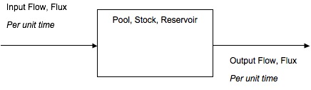
Model Diagrams
All systems that change over time can be described by pools and flows. It is often easiest to understand a system through visual representation. Here is a 1-box stock and flow diagram to show the basic model parts: